LARE-HPA
A Kubernetes autoscaler that dynamically adapts thresholds and cool-downs to the workload.
Mean latency −50.34% vs HPA · ICSOC Distinguished
Before we start
"What percentage should the threshold be?" Autoscaling never had a clean answer to that — so I started from a different question: could the system answer it itself?
A fixed CPU target affects latency and resource use differently as demand changes. I implemented a controller that adjusts the target and downscale retention from observed volatility and trend.
The derivation and experiments are in the LARE-HPA paper under Publications.
Fixed settings could not adapt to demand
A lower HPA CPU target expands capacity earlier but uses more resources. In the paper’s tests, a 60% target used about 22% more CPU than a 90% target. A higher target can delay expansion and increase latency. The controller therefore needed to adapt the setting as demand changed.
If demand rises just after pods are released, the controller must expand again. Keeping them longer avoids some of this repetition but retains unused capacity when demand falls. Both expansion thresholds and release timing needed to adapt.
Forecasting can help, but new applications may lack enough data for offline training. Retraining after changes in demand adds work as well. I chose a model updated from observations collected during execution.
LARE-HPA forecasts load online, adjusts the CPU target from request volatility, and adjusts downscale retention from the trend. It uses observations gathered during execution rather than a separately prepared training dataset.
One Pod, three processes
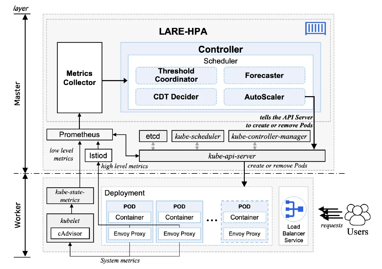
LARE-HPA runs three Python processes in one Pod, handling scaling decisions, threshold adjustment, and cool-down adjustment separately. They share the threshold and retention counter through multiprocessing.Value.
The Metrics Collector queries system and Istio request metrics stored in Prometheus. The Forecaster, Threshold Coordinator, and CDT Decider use them to update predictions and settings; the AutoScaler adjusts Deployment replicas through the Kubernetes API.
Updating forecasts, thresholds, and retention
First, the Forecaster predicts incoming load with an online-learning ARIMA. Classic ARIMA needs enough history and offline training; here the autoregressive coefficients are updated on the fly with Online Newton-Step. It is a second-order optimization that updates the precision matrix (inverse Hessian) in a Sherman-Morrison fashion, so the coefficients track the data as it arrives with no batch retraining. It starts forecasting once 10 lags are available and clamps negative forecasts to zero.
Next, the Threshold Coordinator turns that forecast and recent history into a threshold. It measures volatility as the z-score of the last 10 intervals’ request changes against the full history, then maps it through an inverse sigmoid to a CPU threshold within 5–95%. When volatility is low it raises the threshold to pack pods tighter and save resources; when volatility is high it lowers the threshold to scale earlier and protect QoS.
Finally, the CDT Decider fits a linear regression on the last 60 request intervals and checks residual autocorrelation with the Durbin-Watson statistic. It applies the trend when the statistic falls within the configured acceptance interval of 1.616–2.384. Rising demand lengthens the cool-down counter up to 60 intervals to avoid premature contraction; falling demand shortens it toward 1 to release resources sooner.
Deployment without application code changes
The whole thing runs as a single daemon on a python:3.11-slim image and follows least privilege. It authenticates in-cluster with a dedicated ServiceAccount, and its ClusterRole holds only patch/get/list/watch on deployments/scale and statefulsets/scale plus read access to pods and services.
A ConfigMap defines the target application, Prometheus address, CPU target (75% by default), replica range (1–16), and polling period (60 seconds). A deployment script installs the controller. Separate forecast, threshold, cool-down, and error logs make scaling decisions traceable. Application code remains unchanged, with system and request metrics required in the environment.
Results
Results on a real-world workload (NASA-HTTP trace, 1-second SLO). LARE-HPA cut mean latency from 562.8ms (default HPA) to 279.5ms (95th percentile from 1189.0ms to 600.1ms) and reached 97.24% SLO satisfaction, the highest of the four. It used 638.13 millicores, about 9.5% more than HPA (582.76) but far less than Bi-LSTM (875.85) and Online-BO (1274.75); Online-BO over-provisioned to more than 2× HPA.
| Method | Mean latency | Latency cut | SLO | Resource (mcore) |
|---|---|---|---|---|
| LARE-HPA | 279.5ms | baseline | 97.24% | 638.13 |
| Default HPA | 562.8ms | 50.34% ↓ | 93.86% | 582.76 |
| offline Bi-LSTM | 462.1ms | 39.52% ↓ | 93.06% | 875.85 |
| Online-BO | 519.3ms | 46.18% ↓ | 95.15% | 1274.75 |
Actual values from Table 2 of the paper (latency cut is relative to LARE-HPA). Distinguished Paper (Top 6) at ICSOC 2024.
Wrapping up
The work was named a Distinguished Paper (Top 6) at ICSOC 2024, a top-tier SCIE-class venue; a patent was filed and the software copyright registered, and the code is open-sourced.
The controller updates its forecast from incoming requests without prior training, then adjusts thresholds and retention while evaluating latency and resource use together. The result is a working controller whose settings respond to changing demand rather than remaining fixed.